Tutorial
The microstructural analysis is a powerful, but underused tool of petrostructural analysis. Except acquirement of common statistical parameters, this technique can significantly improve understanding of processes of grain nucleation and grain growth, can bring insights on the role of surface energies or quantify duration of metamorphic and magmatic cooling events as long as appropriate thermodynamical data for studied mineral exist. This technique also allows systematic evaluation of degree of preferred orientations of grain boundaries in conjunction with their frequencies. This may help to better understand the mobility of grain boundaries and precipitations or removal of different mineral phases.
We introduce a new platform, object-oriented Python package PolyLX providing several core routines for data exchange, visualization and analysis of microstructural data, which can be run on any platform supported by Scientific Python environment.
Grains objects
To start working with PolyLX we need to import the polylx package. For our convinience, we can import PolyLX into actual namespace:
[1]:
from polylx import *
To read example data, we can use example method. Note that we create new Grains object, which store all imported Grain features.
[2]:
g = Grains.example()
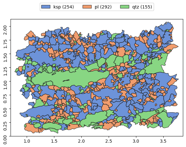
To visualize grain objects from shape file, we can use plot method of Grains object:
[3]:
g.show()
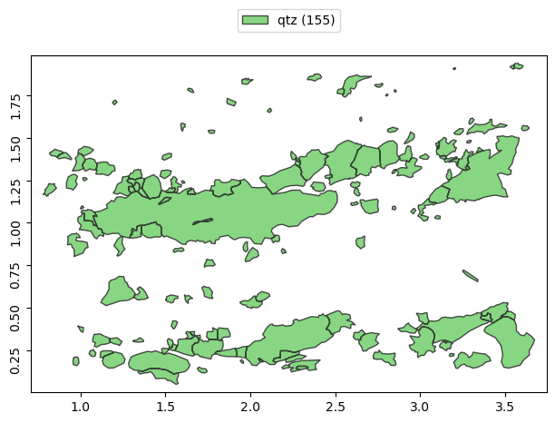
or we can just select Grains by its class name:
[4]:
g['qtz'].show()
The dot notation is used to access individual properties commonly returning values for individual Grain as numpy array.
[5]:
g['qtz'].ar
[5]:
array([1.46370088, 3.55371458, 1.43641139, 1.26293055, 2.10676277,
       1.45200805, 1.98973326, 1.97308557, 2.13420187, 1.76682269,
       1.70083897, 1.38205897, 1.88811465, 1.59948827, 2.50452919,
       1.60296389, 1.4918233 , 2.15318719, 1.27665794, 1.38714959,
       1.67235338, 2.33179583, 1.30609967, 2.73148246, 1.02760669,
       1.33627299, 2.65451284, 1.29069569, 1.73051094, 1.25763409,
       1.90027316, 2.56110638, 1.78555385, 2.40926108, 2.26741705,
       1.71957235, 1.79168709, 1.04770164, 1.293186  , 1.29420065,
       1.48331817, 2.15510614, 2.21246419, 1.57101091, 2.01989715,
       1.1428675 , 2.02888455, 4.07405108, 1.47968881, 1.24770095,
       1.4750185 , 1.37946472, 1.49048108, 1.56668345, 1.43717521,
       1.59756777, 1.58948843, 2.12557437, 2.54316052, 1.98917177,
       1.29809155, 1.70022052, 1.40121941, 1.24674038, 1.50255058,
       1.42880415, 1.73447054, 2.3548111 , 1.52891827, 3.26773221,
       1.33011244, 2.26173396, 3.2151532 , 2.15638456, 1.61602624,
       1.13898611, 2.91625233, 1.94275485, 2.68487563, 1.12446842,
       1.48814907, 1.79425743, 1.19512385, 1.28301942, 1.39853133,
       1.59860483, 3.80709622, 1.75016693, 1.59940152, 1.43972155,
       1.09439109, 2.00023212, 1.87470191, 1.04157011, 1.48561371,
       1.14172901, 1.48211332, 1.52569202, 1.59357336, 1.58054224,
       1.86890813, 1.84729576, 1.45085424, 1.4400654 , 2.6284034 ,
       1.62077026, 1.35218688, 1.69040095, 1.2829313 , 2.7380623 ,
       1.55901231, 1.72569674, 1.18396915, 1.67864861, 2.40971617,
       2.08496427, 2.12907657, 1.20981316, 1.46045276, 1.55428179,
       4.73482949, 2.32570855, 1.95106722, 1.81174297, 4.08295286,
       2.04530043, 1.56215221, 1.42587721, 1.70016792, 1.78887212,
       2.17273986, 2.47995119, 4.59660941, 3.43961286, 3.04193405,
       2.91162332, 2.98790473, 2.55352686, 1.33076709, 7.09385883,
       1.91715238, 1.47161362, 2.39020581, 1.51938795, 1.87839843,
       1.9946499 , 2.27873759, 4.50321651, 5.78162231, 6.9806063 ,
       1.3177092 , 2.33701528, 1.86371784, 1.26166336, 1.28322623])
or we can collect any properties to pandas.DataFrame using df method:
[6]:
g.df('la', 'sa', 'lao', 'sao', 'area', 'length', 'ead', 'ar').head(10)
[6]:
| la | sa | lao | sao | area | length | ead | ar | |
|---|---|---|---|---|---|---|---|---|
| fid | ||||||||
| 0 | 0.066027 | 0.045110 | 70.596636 | 160.596636 | 0.002286 | 0.186196 | 0.053956 | 1.463701 |
| 1 | 0.099033 | 0.057029 | 70.983857 | 160.983857 | 0.004409 | 0.258753 | 0.074922 | 1.736522 |
| 2 | 0.074248 | 0.020893 | 61.438248 | 151.438248 | 0.001123 | 0.175821 | 0.037813 | 3.553715 |
| 3 | 0.045232 | 0.031489 | 85.088587 | 175.088587 | 0.001005 | 0.134427 | 0.035779 | 1.436411 |
| 4 | 0.136445 | 0.108038 | 170.839835 | 80.839835 | 0.011489 | 0.398558 | 0.120948 | 1.262931 |
| 5 | 0.073578 | 0.044938 | 123.223347 | 33.223347 | 0.002471 | 0.201258 | 0.056090 | 1.637319 |
| 6 | 0.103567 | 0.065119 | 149.397514 | 59.397514 | 0.005213 | 0.283110 | 0.081474 | 1.590441 |
| 7 | 0.103189 | 0.077988 | 23.758847 | 113.758847 | 0.005951 | 0.318774 | 0.087048 | 1.323142 |
| 8 | 0.187049 | 0.036611 | 82.108720 | 172.108720 | 0.004407 | 0.404066 | 0.074904 | 5.109041 |
| 9 | 0.270513 | 0.128402 | 76.193288 | 166.193288 | 0.024576 | 0.729051 | 0.176894 | 2.106763 |
[7]:
g.df('ead').describe()
[7]:
| ead | |
|---|---|
| count | 701.000000 |
| mean | 0.072812 |
| std | 0.056812 |
| min | 0.000350 |
| 25% | 0.037140 |
| 50% | 0.058338 |
| 75% | 0.093503 |
| max | 0.638144 |
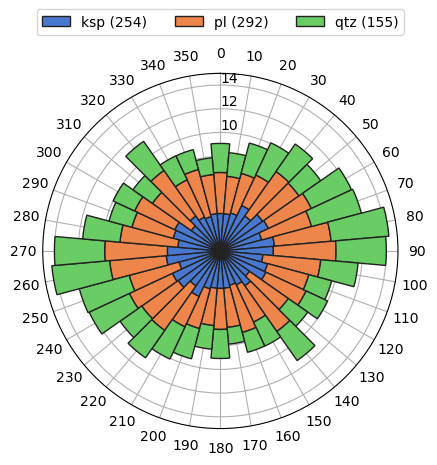
To visualize orientations of objects, we can use rose method:
[8]:
g.rose()
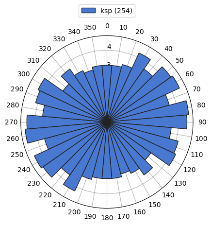
or for just single class:
[9]:
g['ksp'].rose()
To aggregate and summarize multiple properties by different functions according to defined classification (name by default) we can use agg method. Note that cirstat provides functions to calculate various circular statistics.
[10]:
g.agg(
    N=['name', 'count'],
    area=['area', 'sum'],
    mean_ead=['ead', 'mean'],
    mean_or=['lao', circstat.mean],
    spo=['vec', circstat.ot_ar]
)
[10]:
| N | area | mean_ead | mean_or | spo | |
|---|---|---|---|---|---|
| class | |||||
| ksp | 254 | 2.443733 | 0.089710 | 76.875488 | 2.125597 |
| pl | 292 | 1.083516 | 0.060629 | 94.197847 | 1.815966 |
| qtz | 155 | 1.166097 | 0.068071 | 74.320337 | 6.113376 |
The groups method return Pandas GroupBy object which allows any pandas-style manipulation
[11]:
g.groups('ead', 'area', 'la', 'sa').describe().T
[11]:
| class | ksp | pl | qtz | |
|---|---|---|---|---|
| ead | count | 2.540000e+02 | 292.000000 | 1.550000e+02 |
| mean | 8.970974e-02 | 0.060629 | 6.807125e-02 | |
| std | 6.495077e-02 | 0.032438 | 7.054971e-02 | |
| min | 6.641998e-04 | 0.001850 | 3.501464e-04 | |
| 25% | 4.133005e-02 | 0.038226 | 2.970151e-02 | |
| 50% | 7.403298e-02 | 0.053984 | 4.794577e-02 | |
| 75% | 1.191733e-01 | 0.077308 | 7.892656e-02 | |
| max | 4.105520e-01 | 0.190210 | 6.381439e-01 | |
| area | count | 2.540000e+02 | 292.000000 | 1.550000e+02 |
| mean | 9.620995e-03 | 0.003711 | 7.523208e-03 | |
| std | 1.548182e-02 | 0.004170 | 2.778736e-02 | |
| min | 3.464873e-07 | 0.000003 | 9.629176e-08 | |
| 25% | 1.341681e-03 | 0.001148 | 6.930225e-04 | |
| 50% | 4.304819e-03 | 0.002289 | 1.805471e-03 | |
| 75% | 1.115444e-02 | 0.004694 | 4.892680e-03 | |
| max | 1.323812e-01 | 0.028416 | 3.198359e-01 | |
| la | count | 2.540000e+02 | 292.000000 | 1.550000e+02 |
| mean | 1.295772e-01 | 0.086681 | 1.019395e-01 | |
| std | 1.053259e-01 | 0.053220 | 1.366152e-01 | |
| min | 1.013949e-03 | 0.006461 | 1.017291e-03 | |
| 25% | 5.439610e-02 | 0.050202 | 4.314167e-02 | |
| 50% | 9.871911e-02 | 0.072777 | 7.151284e-02 | |
| 75% | 1.793952e-01 | 0.106761 | 1.206513e-01 | |
| max | 8.097226e-01 | 0.279398 | 1.437277e+00 | |
| sa | count | 2.540000e+02 | 292.000000 | 1.550000e+02 |
| mean | 7.545538e-02 | 0.049585 | 5.255111e-02 | |
| std | 5.428555e-02 | 0.027663 | 4.632415e-02 | |
| min | 3.648908e-04 | 0.000583 | 1.457310e-04 | |
| 25% | 3.370683e-02 | 0.031980 | 2.183093e-02 | |
| 50% | 6.643814e-02 | 0.043545 | 3.640605e-02 | |
| 75% | 1.021515e-01 | 0.063468 | 6.490102e-02 | |
| max | 3.252086e-01 | 0.166726 | 3.035541e-01 |
The method classify could be used to define new classification, based on any property and using variety of rules, e.g. 'quantile':
[12]:
g.classify('ar', rule='quantile', k=6)
df = g.df('class', 'name', 'area')
df.head()
[12]:
| class | name | area | |
|---|---|---|---|
| fid | |||
| 0 | 1.45-1.63 | qtz | 0.002286 |
| 1 | 1.63-1.89 | pl | 0.004409 |
| 2 | 2.36-12.16 | qtz | 0.001123 |
| 3 | 1.28-1.45 | qtz | 0.001005 |
| 4 | 1.02-1.28 | qtz | 0.011489 |
To summarize results for individual phases per class we can use pandas pivot table:
[13]:
pd.pivot_table(df,index=['class'], columns=['name'], aggfunc='sum')
[13]:
| area | |||
|---|---|---|---|
| name | ksp | pl | qtz |
| class | |||
| 1.02-1.28 | 0.348379 | 0.158328 | 0.079026 |
| 1.28-1.45 | 0.366220 | 0.176028 | 0.106734 |
| 1.45-1.63 | 0.424773 | 0.163026 | 0.192027 |
| 1.63-1.89 | 0.325575 | 0.157087 | 0.067631 |
| 1.89-2.36 | 0.362103 | 0.226971 | 0.168503 |
| 2.36-12.16 | 0.616684 | 0.202075 | 0.552178 |
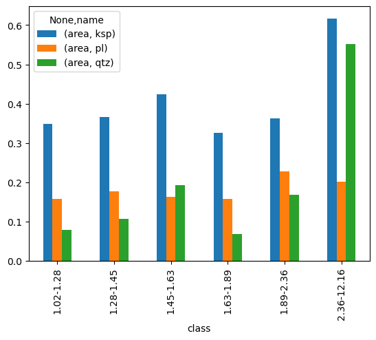
or we can directly plot it..
[14]:
pd.pivot_table(df,index=['class'], columns=['name'], aggfunc='sum').plot(kind='bar');
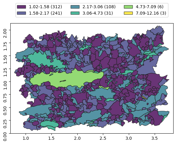
[15]:
g.classify('ar', rule='jenks', k=6)
[16]:
g.show()
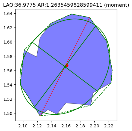
[17]:
g[132].show()
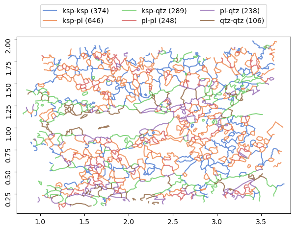
Boundaries objects
The map of grain boundaries could be created from topologically correct grains using boundaries method:
[18]:
b = g.boundaries()
[19]:
b.show()
[20]:
df = b.groups('length').sum()
df['percents']= 100 * df['length'] / df['length'].sum()
df
[20]:
| length | percents | |
|---|---|---|
| class | ||
| ksp-ksp | 23.383974 | 21.384276 |
| ksp-pl | 38.592227 | 35.291983 |
| ksp-qtz | 17.920424 | 16.387946 |
| pl-pl | 11.302490 | 10.335949 |
| pl-qtz | 11.535006 | 10.548581 |
| qtz-qtz | 6.617133 | 6.051264 |
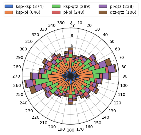
[21]:
b.rose(weights=b.length, scaled=False)
[ ]: