Tutorial
The microstructural analysis is a powerful, but underused tool of petrostructural analysis. Except acquirement of common statistical parameters, this technique can significantly improve understanding of processes of grain nucleation and grain growth, can bring insights on the role of surface energies or quantify duration of metamorphic and magmatic cooling events as long as appropriate thermodynamical data for studied mineral exist. This technique also allows systematic evaluation of degree of preferred orientations of grain boundaries in conjunction with their frequencies. This may help to better understand the mobility of grain boundaries and precipitations or removal of different mineral phases.
We introduce a new platform, object-oriented Python package PolyLX providing several core routines for data exchange, visualization and analysis of microstructural data, which can be run on any platform supported by Scientific Python environment.
Basic usage
To start working with PolyLX we need to import polylx package. For convinience, we will import polylx into actual namespace:
>>> from polylx import *
To read example data, we can use Grains.from_shp method without
arguments. Note that we create new Grains object, which store all
imported features (polygons) from shapefile:
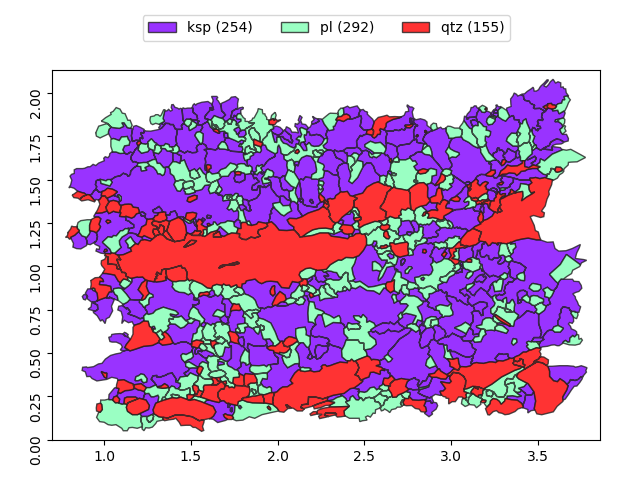
>>> g = Grains.from_shp()
To visualize grain objects from shape file, we can use show method
of Grains object:
>>> g.show()
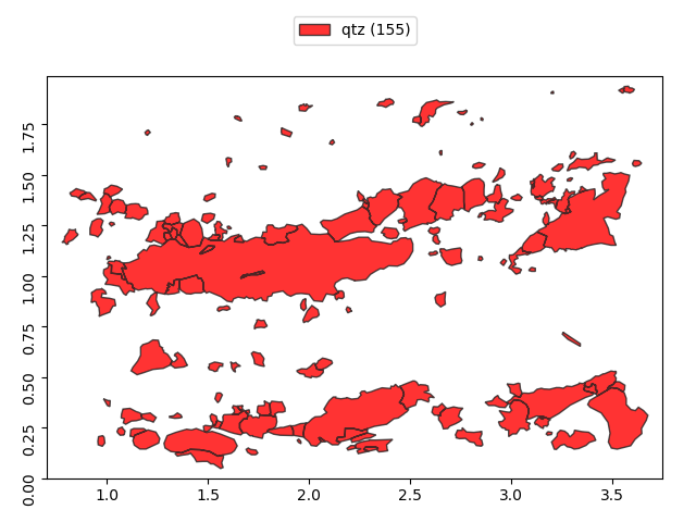
To show only ‘qtz’ phase, we can use fancy indexing:
>>> g['qtz'].show()
Grains support dot notation to access individual properties.
Note that most of properties are returned as numpy.array:
>>> g['qtz'].ar  # get axial ratios
array([ 1.46370088,  3.55371458,  1.43641139,  1.26293055,  2.10676277,
        1.45200805,  1.98973326,  1.97308557,  2.13420187,  1.76682269,
        1.70083897,  1.38205897,  1.88811465,  1.59948827,  2.50452919,
        1.60296389,  1.4918233 ,  2.15318719,  1.27665794,  1.38714959,
        1.67235338,  2.33179583,  1.30609967,  2.73148246,  1.02760669,
        1.33627299,  2.65451284,  1.29069569,  1.73051094,  1.25763409,
        1.90027316,  2.56110638,  1.78555385,  2.40926108,  2.26741705,
        1.71957235,  1.79168709,  1.04770164,  1.293186  ,  1.29420065,
        1.48331817,  2.15510614,  2.21246419,  1.57101091,  2.01989715,
        1.1428675 ,  2.02888455,  4.07405108,  1.47968881,  1.24770095,
        1.4750185 ,  1.37946472,  1.49048108,  1.56668345,  1.43717521,
        1.59756777,  1.58948843,  2.12557437,  2.54316052,  1.98917177,
        1.29809155,  1.70022052,  1.40121941,  1.24674038,  1.50255058,
        1.42880415,  1.73447054,  2.3548111 ,  1.52891827,  3.26773221,
        1.33011244,  2.26173396,  3.2151532 ,  2.15638456,  1.61602624,
        1.13898611,  2.91625233,  1.94275485,  2.68487563,  1.12446842,
        1.48814907,  1.79425743,  1.19512385,  1.28301942,  1.39853133,
        1.59860483,  3.80709622,  1.75016693,  1.59940152,  1.43972155,
        1.09439109,  2.00023212,  1.87470191,  1.04157011,  1.48561371,
        1.14172901,  1.48211332,  1.52569202,  1.59357336,  1.58054224,
        1.86890813,  1.84729576,  1.45085424,  1.4400654 ,  2.6284034 ,
        1.62077026,  1.35218688,  1.69040095,  1.2829313 ,  2.7380623 ,
        1.55901231,  1.72569674,  1.18396915,  1.67864861,  2.40971617,
        2.08496427,  2.12907657,  1.20981316,  1.46045276,  1.55428179,
        4.6980536 ,  2.32570855,  1.95106722,  1.81174297,  4.08295286,
        2.04530043,  1.56215221,  1.42587721,  1.70016792,  1.78887212,
        2.17273986,  2.47995119,  4.59660941,  3.43961286,  3.04193405,
        2.91162332,  2.98790473,  2.55352686,  1.33076709,  7.09385883,
        1.91715238,  1.47161362,  2.39020581,  1.51938795,  1.87839843,
        1.9946499 ,  2.27873759,  4.50321651,  5.78162231,  6.9806063 ,
        1.3177092 ,  2.33701528,  1.86371784,  1.26166336,  1.28322623])
More conviniet way to work with Grains attributes is collect any properties
to pandas.DataFrame using df method:
>>> g.df('la', 'sa', 'lao', 'area', 'length', 'ead', 'ar').head(10)
           la        sa         lao      area    length       ead        ar
fid
0    0.066027  0.045110   70.596636  0.002286  0.186196  0.053956  1.463701
1    0.099033  0.057029   70.983857  0.004409  0.258753  0.074922  1.736522
2    0.074248  0.020893   61.438248  0.001123  0.175821  0.037813  3.553715
3    0.045232  0.031489   85.088587  0.001005  0.134427  0.035779  1.436411
4    0.136445  0.108038  170.839835  0.011489  0.398558  0.120948  1.262931
5    0.073578  0.044938  123.223347  0.002471  0.201258  0.056090  1.637319
6    0.103567  0.065119  149.397514  0.005213  0.283110  0.081474  1.590441
7    0.103189  0.077988   23.758847  0.005951  0.318774  0.087048  1.323142
8    0.187049  0.036611   82.108720  0.004407  0.404066  0.074904  5.109041
9    0.270513  0.128402   76.193288  0.024576  0.729051  0.176894  2.106763
Once you have pandas.DataFrame, check pandas manual to what you can do.
Here is fe examples:
>>> g.df('ead').describe()
              ead
count  701.000000
mean     0.072812
std      0.056812
min      0.000350
25%      0.037140
50%      0.058338
75%      0.093503
max      0.638144
agg method aggregate properties according to defined classification
(name by default):
>>> g.agg('area','sum', 'ead', 'mean', 'name', 'count')
                area       ead  name
name_class
ksp         2.443733  0.089710   254
pl          1.083516  0.060629   292
qtz         1.166097  0.068071   155
The groups method return pandas.GroupBy object which allows any
pandas-style manipulation:
>>> g.groups('ead', 'area', 'la', 'sa').describe().T
name_class           ksp          pl           qtz
area count  2.540000e+02  292.000000  1.550000e+02
     mean   9.620995e-03    0.003711  7.523208e-03
     std    1.548182e-02    0.004170  2.778736e-02
     min    3.464873e-07    0.000003  9.629176e-08
     25%    1.341681e-03    0.001148  6.930225e-04
     50%    4.304819e-03    0.002289  1.805471e-03
     75%    1.115444e-02    0.004694  4.892680e-03
     max    1.323812e-01    0.028416  3.198359e-01
ead  count  2.540000e+02  292.000000  1.550000e+02
     mean   8.970974e-02    0.060629  6.807125e-02
     std    6.495077e-02    0.032438  7.054971e-02
     min    6.641998e-04    0.001850  3.501464e-04
     25%    4.133005e-02    0.038226  2.970151e-02
     50%    7.403298e-02    0.053984  4.794577e-02
     75%    1.191733e-01    0.077308  7.892656e-02
     max    4.105520e-01    0.190210  6.381439e-01
la   count  2.540000e+02  292.000000  1.550000e+02
     mean   1.295772e-01    0.086681  1.019395e-01
     std    1.053259e-01    0.053220  1.366152e-01
     min    1.013949e-03    0.006461  1.017291e-03
     25%    5.439610e-02    0.050202  4.314167e-02
     50%    9.871911e-02    0.072777  7.151284e-02
     75%    1.793952e-01    0.106761  1.206513e-01
     max    8.097226e-01    0.279398  1.437277e+00
sa   count  2.540000e+02  292.000000  1.550000e+02
     mean   7.545538e-02    0.049585  5.255111e-02
     std    5.428555e-02    0.027663  4.632415e-02
     min    3.648908e-04    0.000583  1.457310e-04
     25%    3.370683e-02    0.031980  2.183093e-02
     50%    6.643814e-02    0.043545  3.640605e-02
     75%    1.021515e-01    0.063468  6.490102e-02
     max    3.252086e-01    0.166726  3.035541e-01
The classify method could be used to define new classification, based
on any property and using variety of methods:
>>> g.classify('ead', k=6)
>>> df = g.df('class', 'name', 'area')
>>> df.head()
       ead_class name      area
fid
0    0.048-0.066  qtz  0.002286
1    0.066-0.091   pl  0.004409
2    0.030-0.048  qtz  0.001123
3    0.030-0.048  qtz  0.001005
4    0.091-0.141  qtz  0.011489
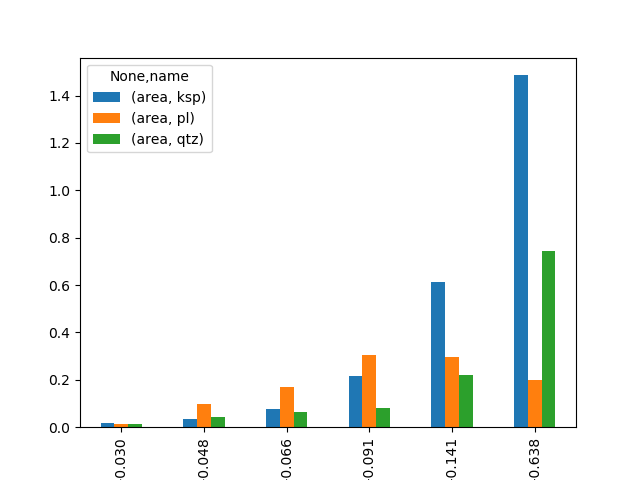
To summarize results for individual phases per class we can use
pandas.pivot_table:
>>> pd.pivot_table(df,index=['ead_class'], columns=['name'], aggfunc=np.sum)
                 area
name              ksp        pl       qtz
ead_class
0.000-0.030  0.017510  0.015057  0.015377
0.030-0.048  0.035587  0.096870  0.043866
0.048-0.066  0.077185  0.170371  0.065184
0.066-0.091  0.214921  0.305016  0.079672
0.091-0.141  0.612776  0.296543  0.218996
0.141-0.638  1.485754  0.199659  0.743003
or we can directly plot it:
>>> pd.pivot_table(df,index=['ead_class'], columns=['name'], aggfunc=np.sum).plot(kind='bar')
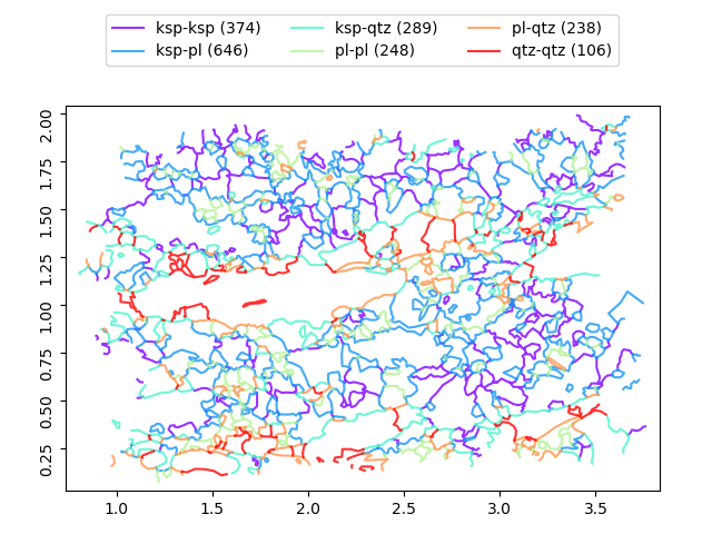
Work with boundaries
The Boundaries object could be created from grains with correct
topology (use OpenJUMP, QGIS or ArcGIS to validate grain shapefile topology):
>>> b = g.boundaries()
>>> b.show()
Most of methods and properties demonstrated for Grains are valid also
for boundaries:
>>> b.agg('sum', 'length')
               length
name_class
ksp-ksp     23.383974
ksp-pl      38.592227
ksp-qtz     17.920424
pl-pl       11.302490
pl-qtz      11.535006
qtz-qtz      6.617133